
The Science of Offshore Wind: Why Sea Winds Are Powerful
Offshore wind resources can be strong and relatively consistent because open water usually presents less surface drag than forests, buildings or complex terrain, while large weather systems can travel over a long marine fetch with fewer abrupt obstacles. At turbine height, however, the result depends on atmospheric stability, air–sea temperature differences, wind direction, waves, distance from shore, season and storms. Sea winds are not automatically stronger at every place or time.
That qualification matters. In weather forecasting, an offshore wind can simply mean wind blowing from land toward the sea. In wind energy, the phrase usually refers to the wind resource over water. Developers therefore assess the actual wind climate across the full rotor, not a generic coastal impression or a single average speed. The U.S. Department of Energy’s wind resource assessment programme combines long-term models with measurements of wind at multiple heights, direction, air and sea-surface temperature, waves and currents.
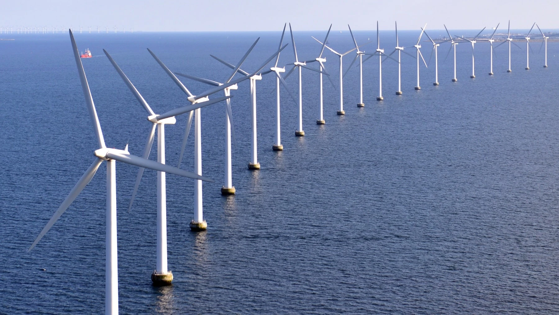
Why open water changes the wind profile
Wind near any surface loses momentum through friction. Trees, buildings and terrain create comparatively large aerodynamic roughness and turbulence. The sea is generally smoother, so the near-surface flow often experiences less drag and retains more speed. But the ocean is not frictionless: waves change roughness and exchange momentum with the air. The Met Office’s coupled ocean modelling explanation notes that predicted wave roughness affects atmospheric wind speed as well as heat, moisture and momentum exchange.
Fetch is the distance wind travels over a surface. A long marine fetch can allow the flow to adjust to ocean conditions, while a short fetch near shore may retain a land-influenced internal boundary layer. Coastlines, headlands, islands and coastal hills can accelerate, shelter, turn or channel the flow. Sea-breeze circulations caused by land–sea heating contrasts can add a daily pattern, but they are not constant engines: cloud, season, coastline shape and the larger weather situation can strengthen, shift or suppress them.
Stability, temperature gradients and wind shear
The marine atmospheric boundary layer is the part of the atmosphere directly influenced by the sea. When warm air moves over cooler water, the lower layer often becomes stable: vertical mixing is suppressed, wind speed can change sharply with height, and low-level jets may form. When cold air passes over warmer water, buoyant mixing can make the layer unstable, redistributing momentum vertically and producing a different shear and turbulence profile. Neutral conditions sit between these cases.
Wind shear is the change of wind speed or direction with height. A modern offshore rotor samples a deep slice of the boundary layer, so the blade tip at the top may experience different speed and direction from the blade tip at the bottom. That affects energy capture, cyclic loading and wakes. The NOAA-hosted peer-reviewed review Scientific challenges to characterizing the wind resource in the marine atmospheric boundary layer identifies shear, stability, low-level jets, waves and coastal processes as linked measurement and modelling challenges—not details that one average wind speed can represent.
Hub height matters because it places the rotor in a different part of that vertical profile, not because wind must increase uniformly with height. A taller hub may reach a better resource at one site, a jet maximum at another, or a strongly sheared layer that increases loads. This is why wind farm location and micrositing studies use height-resolved measurements and site-specific models.
What the wind-speed-cubed rule really means
For a simplified stream of air, available aerodynamic power can be written as P = ½ρAv³: air density ρ, swept area A and wind speed v. Holding the other terms constant, available power varies with the cube of wind speed. The DOE wind guidebook presents this relationship with a power coefficient for the fraction a rotor can capture. It is a useful sensitivity rule, not a promise that a 10% increase in measured wind will always produce 33% more electrical energy.
Real turbines follow model-specific power curves. Below cut-in speed they do not generate; between cut-in and rated speed output rises; above rated speed control systems limit output; and at the cut-out threshold the turbine may stop to protect equipment. DOE’s severe-weather explanation and power curve shows why extreme wind does not equal unlimited generation. Storms can provide high wind speeds while also creating gusts, turbulence, waves, shutdowns and inaccessible conditions.
| Common claim | What the science supports | Project implication |
|---|---|---|
| Sea winds are always stronger | Lower roughness often helps, but stability, fetch, coastlines, waves and weather determine the local result. | Measure the site and full rotor layer. |
| Power always follows v³ | The cubic relationship describes available aerodynamic power under simplified assumptions. | Use the actual turbine power curve and loss model for energy yield. |
| The strongest wind is the best wind | Extreme winds can cause high loads, rough seas and protective shutdowns. | Assess design extremes, availability and access—not only mean speed. |
| Open water means no turbulence | Waves, stability, fronts, storms and turbine wakes all generate or modify turbulence. | Model loads and wakes across representative conditions. |
From resource quality to spacing and wakes
A turbine extracts momentum and leaves slower, often more turbulent air downstream. Spacing and row orientation are therefore optimised against the directional wind climate, lease boundary, foundations, cables, installation and maintenance access—not selected by one universal rotor-diameter rule. Stable atmospheric conditions can allow wake deficits to persist farther because weaker mixing replenishes momentum more slowly; unstable conditions often mix wakes out faster. NREL’s offshore wind modelling assumptions explicitly calculate wake losses from site-specific resource data and caution that turbulence depends on atmospheric conditions.
The net resource is what remains after wake, electrical, availability, curtailment and other losses. Larger spacing may reduce some wake interactions but lengthen array cables and transit routes and use more seabed area. The optimum layout is therefore a system trade-off. A nearby project can also alter the incoming flow, so regional build-out belongs in cumulative wake assessment.
Why wind science also shapes access and O&M
A productive wind climate and a workable maintenance climate are related but not identical. The same weather system that raises output can increase wave height, vessel motion, transfer risk, blade loading and the chance of a turbine shutdown. Wind direction and fetch influence sea state; wave period, current, visibility and lightning may constrain work even when mean wind speed appears acceptable. Weather windows must therefore be defined for the vessel, transfer system, turbine state, task and rescue method.
Resource and metocean data feed vessel strategy, technician scheduling, spares, inspection timing and expected downtime. The practical chain runs from forecast to access decision to completed scope. Gridinta’s guide to CTV, SOV and walk-to-work access compares operating concepts, while offshore maintenance campaign planning explains how task readiness and weather-window logic should be joined.
For owners and operators, a good wind resource only creates value when turbines remain available and work can be executed safely. Defined offshore wind farm maintenance scopes connect inspections, repairs and access planning to the real site conditions rather than to assumptions about a uniformly smooth or predictable sea. The offshore-versus-onshore maintenance comparison shows how marine access, exposure and emergency response turn those conditions into a different operating model.